
RTM (regression to the mean)
RTM is the BIG effect at speed camera sites.
The authorities have estimated that RTM is the largest effect at speed camera sites, but they haven’t found a method to remove it.
This means that they have never established the effect of their speed cameras.
I therefore developed the FTP (four time periods) method.
My new method is capable of:
- measuring RTM.
- completely removing RTM from results.
I also developed a new more accurate method to compensate for trend.
I then applied my FTP method to produce the first speed camera report that did not have RTM in the results.
This is the most accurate report on the effect of speed cameras anywhere in the world.
- 2008: I published my FTP method (and method for trend).
- 2009: I received the official database of collisions at speed camera sites in Thames Valley.
- 2012: I published the 1st report to use the FTP method (Report).
- 2013: My report is reviewed and accepted into the Road Safety Knowledge Centre.
- 2013: My FTP method is endorsed by the DfT (department for transport) and RAC foundation.
4.1 What is RTM?
RTM stands for “regression to the mean” and it’s just a fancy way of saying “return to normal”.
It occurs when we have a random variable and a selection process.
Random variable:
If we roll a dice 100 times and add up the numbers, we should get a total of around 350.
This is because the average per roll of a dice is 3.5 and this value is called the “mean”.
Selection process:
If we now keep rolling the dice until we get a “6” and then install a camera, the next roll of the dice would generally be lower than 6. If we installed lots of cameras, each one after rolling a 6, the average before the cameras would be 6, and the average after should be around 3.5. This change (from 6 to 3.5) is called “regression to the mean”.
- RTM is the change that occurs in a random variable from a “selected or known” value, to it’s “normal or expected” value.
Speed cameras:
When camera sites are selected following an unusually high collision rate, we would expect a reduction due to RTM. This reduction occurs at the end of the selection process but it then takes quite some time before the cameras are installed. It’s the timing that’s important because it allows us to separate the effect of the cameras, from that of RTM.
- RTM occurs before the cameras are installed, whereas the cameras can only have an effect after.
4.2 How big is RTM in official reports?
Most official reports don’t even mention RTM, but 2 of the largest did attempt to make an estimate:
- RTM is estimated to be larger than all other factors combined (the 4YE national safety camera programme).
- RTM is indicated to be larger than all other factors (the RAC foundation report 2010).
Both of these reports suggest that:
- RTM is so huge that it should be obvious in the data (it should stick out like a sore thumb).
- RTM needs to be fully excluded from results in order to find the much smaller effect of the cameras.
Despite RTM being so obvious, the speed camera operators have refused to deal with it.
- Not a single official report has fully excluded RTM from their results.
4.3 Can the effects of speed cameras be determined directly (without having to consider RTM)?
Yes, just run scientific trials known as RCTs. These would give a direct answer to the question:
“What effect do speed cameras have on the roads where they operate”?
If RCTs were run, there would be no need for any of the evaluations of RTM at speed camera sites and no need for the prolonged confusion and debate over what effect speed cameras actually have.
- The speed camera operators have never run scientific trials, and still refuse to do so (scientific trials).
4.4 What factors influence collision rates at speed camera sites?
Most reports compare collision rates before and after cameras were installed and then assume that the cameras caused the difference. This is not true, however, as several factors are involved. The main ones are:
- RTM.
- Trend (area-wide effects, such as increasing traffic flow, improved vehicle safety, etc).
- The speed cameras.
We know the combined effect of all of these factors (just read any official report) but the effect of RTM and trend need to be removed so that what is left is the effect of the speed cameras. No official report has ever done this.
Note, collision rates can also change due to co-intervention (other measures installed) and diversion of traffic.
4.5 The theory of the FTP method.
Download: spreadsheet (3 pages)
We start by performing a site-selection process.
Consider a theoretical county called “Oxbube” where collisions are generated randomly. We then select where we are going to use “imaginary speed cameras” and the results are examined.
On page 4.3 there is a database with 300 rows and 9 columns. Each row represents a road and each column represents a year. Each cell in the database is given a 0, 1 or 2 generated randomly. This gives a mean rate of 1 collision per year per site.
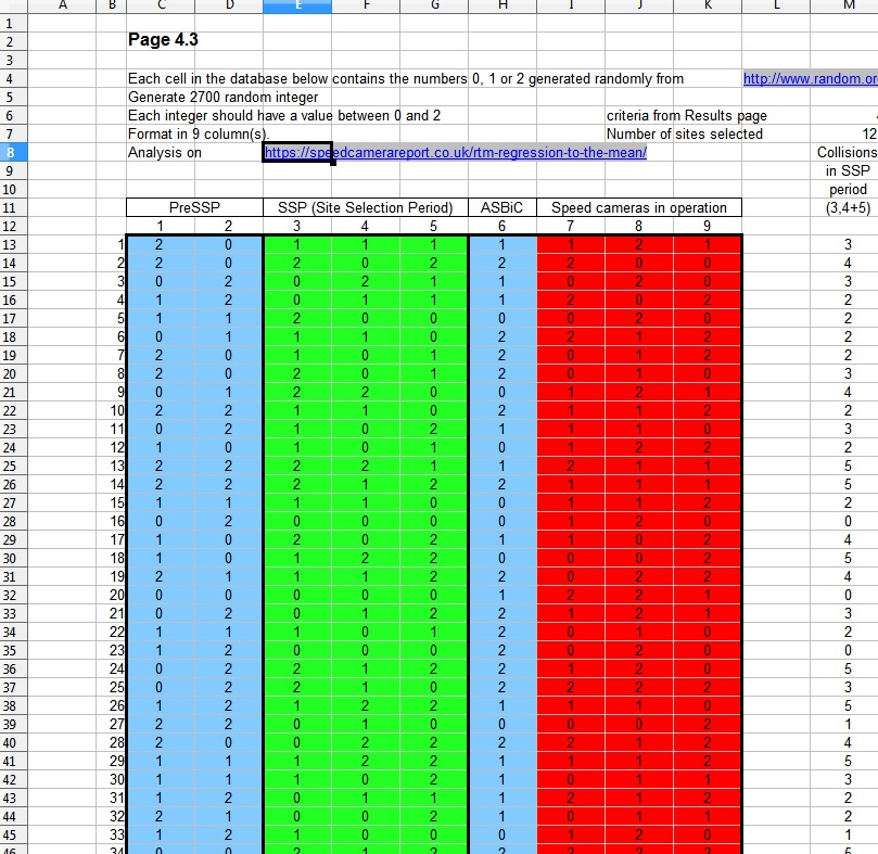
The SSP (Site Selection Period) is years 3, 4 and 5. If a road had 4 or more collisions during that time, it is called a “collision hot-spot” and designated a speed camera site.
Year 6 represents the delay before the cameras are installed and the imaginary speed cameras are operating from the start of year 7.
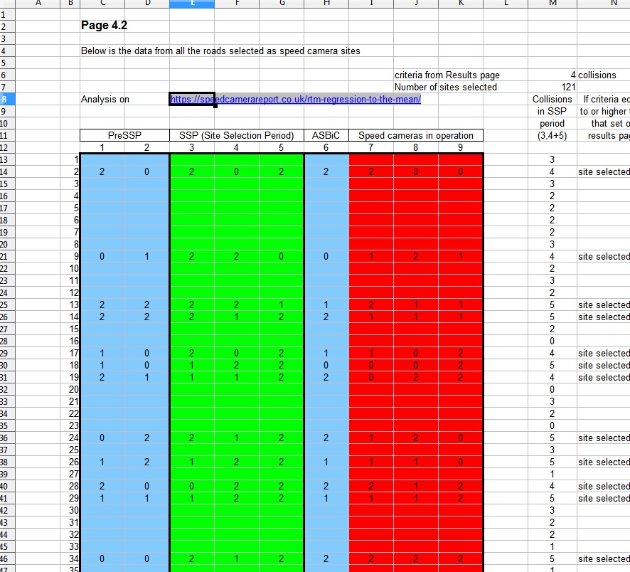
On page 4.2 is the same database but only showing the sites selected for speed cameras.
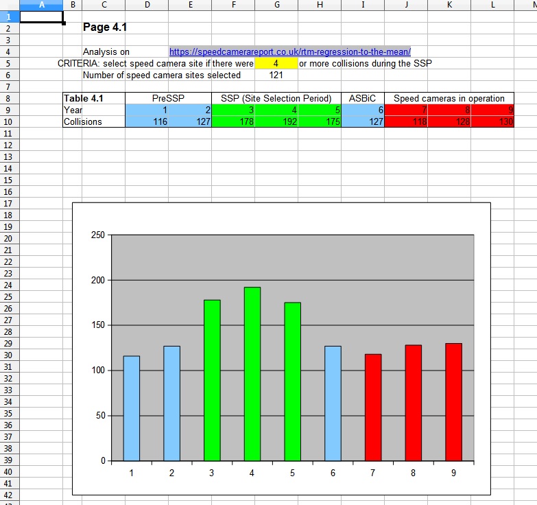
Page 4.1 has the results. Table 4.1 shows the total number of collisions at all of the selected sites in each of the 9 years. Below it is a graph of those numbers.
The graph clearly shows a large reduction in collisions at these sites.
Comparing 3 years after the cameras, to the 3 year SSP before, there was a 31% reduction.
The Oxbube cameras, though, cannot influence randomly generated numbers therefore it must be something else that caused the 31% reduction.
This is the effect known as RTM.
4.6 The Oxbube camera sites.
Figure 4.1 shows the same data as the graph on Page 4.1 but it is labelled to show the relevant features. The data falls into 4 time periods:
- PreSSP (blue).
- SSP (green).
- ASBiC (blue).
- With speed cameras (red).
There are 121 camera sites therefore a mean rate of 121 collisions per year (1 per site per year).
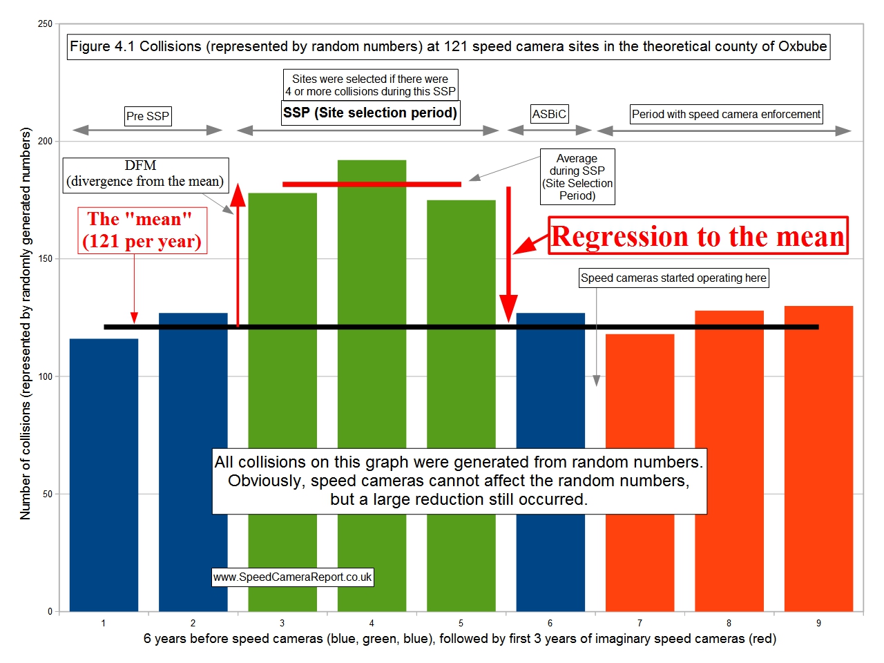
These are the features of the site selection process that can be seen in Figure 4.1:
- Collisions did not occur at their “mean” rate during the SSP.
- Collisions did occur at around their “mean” rate in the other 3 periods (PreSSP, ASBiC and with cameras).
- RTM occurs at the end of the SSP.
- RTM is not a gradual change, it is sudden (vertical).
- DFM (divergence from the mean) occurs at the start of the SSP.
- DFM is similar in size to RTM, but in the opposite direction. It is also a sudden change.
4.7 Identifying the SSP.
To identify the SSP at real camera sites, we look for the same features in the data as are seen in Figure 4.1. This means splitting the data before cameras into 3 time periods where:
- the 1st and 3rd have a similar collision rate.
- the 2nd has a rate different to the 1st and 3rd (this is the SSP).
- The 2nd should be a duration similar to commonly used SSPs (3 to 5 years).
- the change from the 1st to the 2nd should be sudden (vertical)
- the change from the 2nd to the 3rd should also be sudden (this is RTM).
If all 5 of these occur in a graph of collisions at real camera sites, then the 2nd period has been correctly identified as the SSP for those sites.
4.8 New method to compensate for “trend”.
The standard method is to take an average of the change in collisions over the whole area, and apply that to results at the camera sites. The problem is that this can be less accurate over longer time periods (as might be needed in the FTP method) and cannot deal with sudden changes (as occurred in Thames Valley in 1999).
I therefore developed a new method that is more accurate:
- Compensates for trend as it changes both up and down over very long time periods.
- Automatically compensates for sudden changes.
- Doesn’t use estimates or approximate values.
To apply this new method simply:
- Create a new database.
- Convert each item of collision data to it’s percentage of the area-wide total.
- ie 100 x number of collisions / area-wide total in the same time period.
- Put the answers into your new database.
Your new database contains collision rates at sites relative to the whole area.
This database therefore produces results that are automatically compensated for trend.
4.9 The FTP method.
Essentially, the FTP method reverse engineers the site-selection process.
(the following assumes your database contains rows for data at each site and columns for consecutive time periods).
I invented these 3 names for the time periods before cameras:
PreSSP: before the SSP.
SSP: site selection period.
ASBiC: after the SSP but before intervention commences.
To find the “mean” % rate before cameras:
- Start with your database of % collisions (to compensate for trend, see 4.8).
- Mark the installation date of the 1st site and move the data for every other site left or right such that their installation date lines up with the 1st.
- Note, this changes the columns from absolute time periods, to relative time periods.
- Note, this is standard practice in official reports, it’s how 3 years before and after is calculated.
- Plot the addition of the data in each column on a graph.
- Examine the graph to identify the start and end of the SSP (see 4.7).
- This gives you the PreSSP and ASBiC periods.
- Calculate the “mean” % rate before cameras by combining the data in the PreSSP and ASBiC periods.
- The final result is the % rate after cameras, compared to the “mean” % rate before.
If the SSP has been correctly identified, then the result of the FTP method is the change that occurred at the camera sites, compensated for trend and without any RTM.
- My FTP method produces the most accurate evaluation of the effect of speed cameras that it is possible to achieve, given the data available.
This is the 1st report to use the FTP method (Report).
